Estimate Cyclic Trends in Gene Expression Levels Using B-splines

fit_bspline(yy, time)

Arguments

yy	A vector of gene expression values for one gene. The expression values are assumed to have been normalized and transformed to standard normal distribution.
time	A vector of angles (cell cycle phase).

Value

A list with two elements: pred.yy, the estimated cyclic trend; pve, proportion of variance in gene expression levels explained by the cyclic trend.

Examples

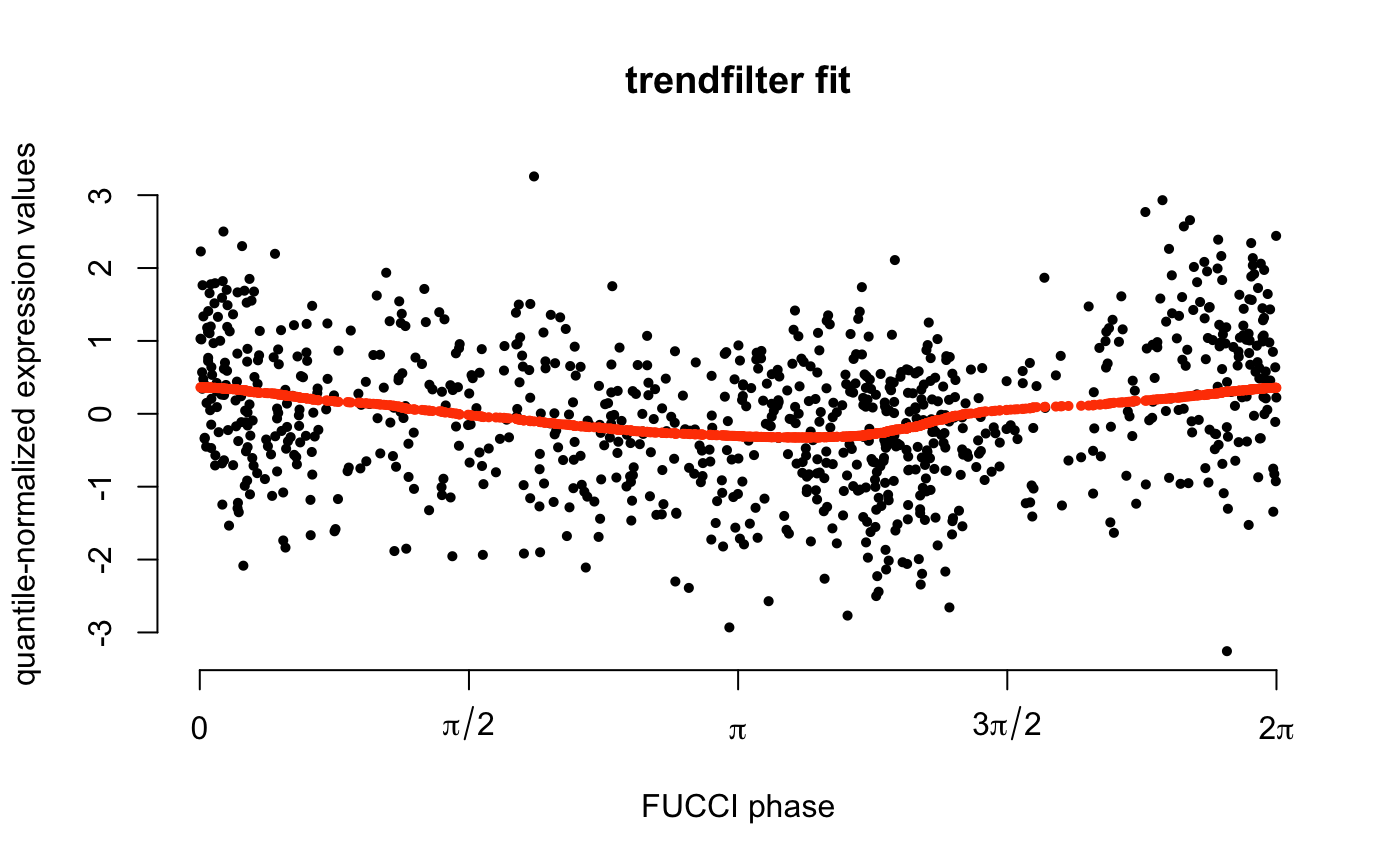
library(SingleCellExperiment)
data(sce_top101genes)

# Select top 10 cyclic genes.
sce_top10 <- sce_top101genes[order(rowData(sce_top101genes)$pve_fucci,
                                   decreasing=TRUE)[1:10],]
coldata <- colData(sce_top10)

# Get ccell cycle phase based on FUCCI scores.
theta <- coldata$theta
names(theta) <- rownames(coldata)

# Normalize expression counts.
sce_top10 <- data_transform_quantile(sce_top10, ncores=2)
#> computing with 2 threads
exprs_quant <- assay(sce_top10, "cpm_quantNormed")

# Order FUCCI phase and expression.
theta_ordered <- theta[order(theta)]
yy_ordered <- exprs_quant[1, names(theta_ordered)]

fit <- fit_trendfilter(yy_ordered)
#> Fold 1 ... Fold 2 ... Fold 3 ... Fold 4 ... Fold 5 ... 

plot(x=theta_ordered, y=yy_ordered, pch=16, cex=0.7, axes=FALSE,
  ylab="quantile-normalized expression values", xlab="FUCCI phase",
  main = "trendfilter fit")
points(x=theta_ordered, y=fit$trend.yy, col="orangered", pch=16, cex=0.7)
axis(2)
axis(1,at=seq(0,2*pi,pi/2),
     labels=c(0,expression(pi/2), expression(pi), expression(3*pi/2),
              expression(2*pi)))