Evaluation criteria

Calibrarion

We say that a method is well-calibrated if for all genes identified as significant at a given cut-off, most of the genes are true effects. Take s-value for an example, of all genes assigned a s-value < .05, we would expect that 95 percent of the genes are truly differently expressed and correctly signed. Take q-value for an example, of all genes assigned a q-value < .05, we would expect that 95% of the genes are truly differently expressed (though not necessary correctly signed) in a well-calibrated method.

Power

We say that a method performs well in power if the method is able to differentiate between null and non-null genes (in datasets that contain both null and non-null genes). Generally speaking, a method that performs in power returns more significant calls among non-null genes than among null genes.

The common approach to evaluate power is computing area under the curve of sensitivty versus specificity (ROC curve). In a ROC curve, the true positive rate (sensitivity) is plotted as a function of the false positive rate (1-specificity). We say tht a method is well-performed if true positive rate is consistently higher than false positive rate at different thresholds of false positive rate.

Below I make a simulation data to demonstrate the calculations of true positive rate and false positive rate.

library(ashbun)

# load iPSC raw counts
library(singleCellRNASeqHumanTungiPSC)

Loading required package: Biobase

Loading required package: BiocGenerics

Loading required package: parallel

Attaching package: 'BiocGenerics'

The following objects are masked from 'package:parallel':

    clusterApply, clusterApplyLB, clusterCall, clusterEvalQ,
    clusterExport, clusterMap, parApply, parCapply, parLapply,
    parLapplyLB, parRapply, parSapply, parSapplyLB

The following objects are masked from 'package:stats':

    IQR, mad, sd, var, xtabs

The following objects are masked from 'package:base':

    anyDuplicated, append, as.data.frame, cbind, colMeans,
    colnames, colSums, do.call, duplicated, eval, evalq, Filter,
    Find, get, grep, grepl, intersect, is.unsorted, lapply,
    lengths, Map, mapply, match, mget, order, paste, pmax,
    pmax.int, pmin, pmin.int, Position, rank, rbind, Reduce,
    rowMeans, rownames, rowSums, sapply, setdiff, sort, table,
    tapply, union, unique, unsplit, which, which.max, which.min

Welcome to Bioconductor

    Vignettes contain introductory material; view with
    'browseVignettes()'. To cite Bioconductor, see
    'citation("Biobase")', and for packages 'citation("pkgname")'.

data <- get(data("HumanTungiPSC"))
data_sub <- exprs(data)[,pData(data)$individual == "NA19239"]

# generate a simulated data with bignormal prior
set.seed(999)
simdata_list <- simulationWrapper(data_sub, Nsim = 1,
                                  Ngenes = 500,
                                  Nsamples = 30,
                                  sample_method = "all_genes",
                                  pi0 = .5,
                                  beta_args = args.big_normal(betapi = 1,
                                                              betamu = 0, betasd = .8))

# fitting limmaVoom 
results.limmaVoom <- ashbun::methodWrapper.limmaVoom(counts = simdata_list[[1]]$counts, 
                                                     condition = simdata_list[[1]]$condition)

Warning: package 'limma' was built under R version 3.4.2

# fitting ash
library(ashr)
results.limmaVoomAsh <- ash(results.limmaVoom$betahat,
                            results.limmaVoom$sebetahat)

# compute ROC curve
roc.data <- data.frame(nonnull = 1- simdata_list[[1]]$is_nullgene, 
                       pvalue.limmaVoom = results.limmaVoom$pvalue,
                       lfsr.limmaVoomAsh = results.limmaVoomAsh$result$lfsr)

# true positive rate and false positive rate
roc.data_limmaVoom <- 
  data.frame(method = "limmaVoom",
             cutoff = quantile(roc.data$pvalue.limmaVoom, prob = c(.1, .3, .5, .7, .9)))
for (index in 1:length(roc.data_limmaVoom$cutoff)) {
  cutoff <- roc.data_limmaVoom$cutoff[index]
  roc.data_limmaVoom$sensitivity[index] <- 
    with(roc.data, sum(nonnull == 1 & pvalue.limmaVoom < cutoff)/sum(pvalue.limmaVoom < cutoff))
  roc.data_limmaVoom$specificity[index] <- 
    with(roc.data, sum(nonnull == 0 & pvalue.limmaVoom > cutoff)/sum(pvalue.limmaVoom > cutoff))
}

roc.data_limmaVoomAsh <- 
  data.frame(method = "limmaVoomAsh",
             cutoff = quantile(roc.data$lfsr.limmaVoomAsh, prob = c(.1, .3, .5, .7, .9)))
for (index in 1:length(roc.data_limmaVoomAsh$cutoff)) {
  cutoff <- roc.data_limmaVoomAsh$cutoff[index]
  roc.data_limmaVoomAsh$sensitivity[index] <- 
    with(roc.data, sum(nonnull == 1 & lfsr.limmaVoomAsh < cutoff)/sum(lfsr.limmaVoomAsh < cutoff))
  roc.data_limmaVoomAsh$specificity[index] <- 
    with(roc.data, sum(nonnull == 0 & lfsr.limmaVoomAsh > cutoff)/sum(lfsr.limmaVoomAsh > cutoff))
}

library(ggplot2)
roc.plot <- rbind(roc.data_limmaVoom, roc.data_limmaVoomAsh)
ggplot(roc.plot, aes(x = 1- specificity,
                     y = sensitivity, col = method)) + geom_line()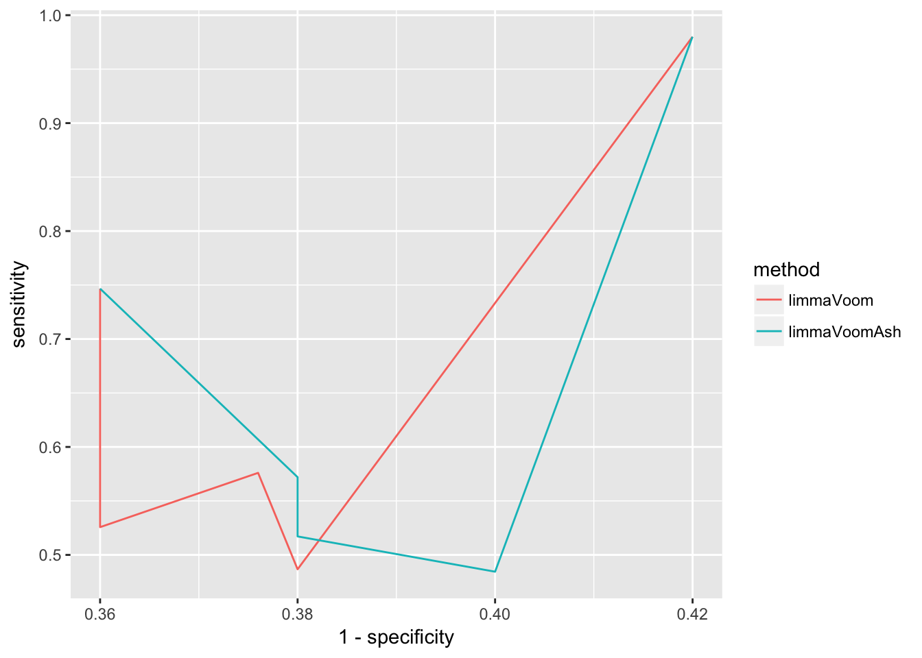 

The above plot is based on 5 cutoffs of specificity and covers only a narrow range of the relationships between true positive rate and false positive rate (1-specificity). pROC package provides a convenient function to compute true positive rate as a function of false positive rate between the values of 0 to 1.

Interpretation: First, we observe that the results are well above chance occurrence - that is, the two lines are above the line wherein sensitivity equals 1-specificity, indicating that the number of true/false cases are above the same in significant and non-significant calls and hence the data is not well suited for method performance evaluation. Second, we focus on the low value range of 1-specificity - for example, at false positive rate of .25 (among non-significant calls, 25% are wrongly called as significant), true positive rate is slightly above .5 for both methods.

roc.pROC_limmaVoom <- pROC::roc(response = roc.data$nonnull, 
                                predictor = roc.data$pvalue.limmaVoom)
roc.pROC_limmaVoomAsh <- pROC::roc(response = roc.data$nonnull, 
                                   predictor = roc.data$lfsr.limmaVoomAsh)

roc.plot_pROC <- rbind(
  data.frame(method = "limmaVoom",
             sensitivity = roc.pROC_limmaVoom$sensitivities,
             specificity = roc.pROC_limmaVoom$specificities),
  data.frame(method = "limmaVoomAsh",
           sensitivity = roc.pROC_limmaVoomAsh$sensitivities,
           specificity = roc.pROC_limmaVoomAsh$specificities) )

library(ggplot2)
ggplot(roc.plot_pROC, aes(x = 1- specificity,
                     y = sensitivity, col = method)) + geom_line()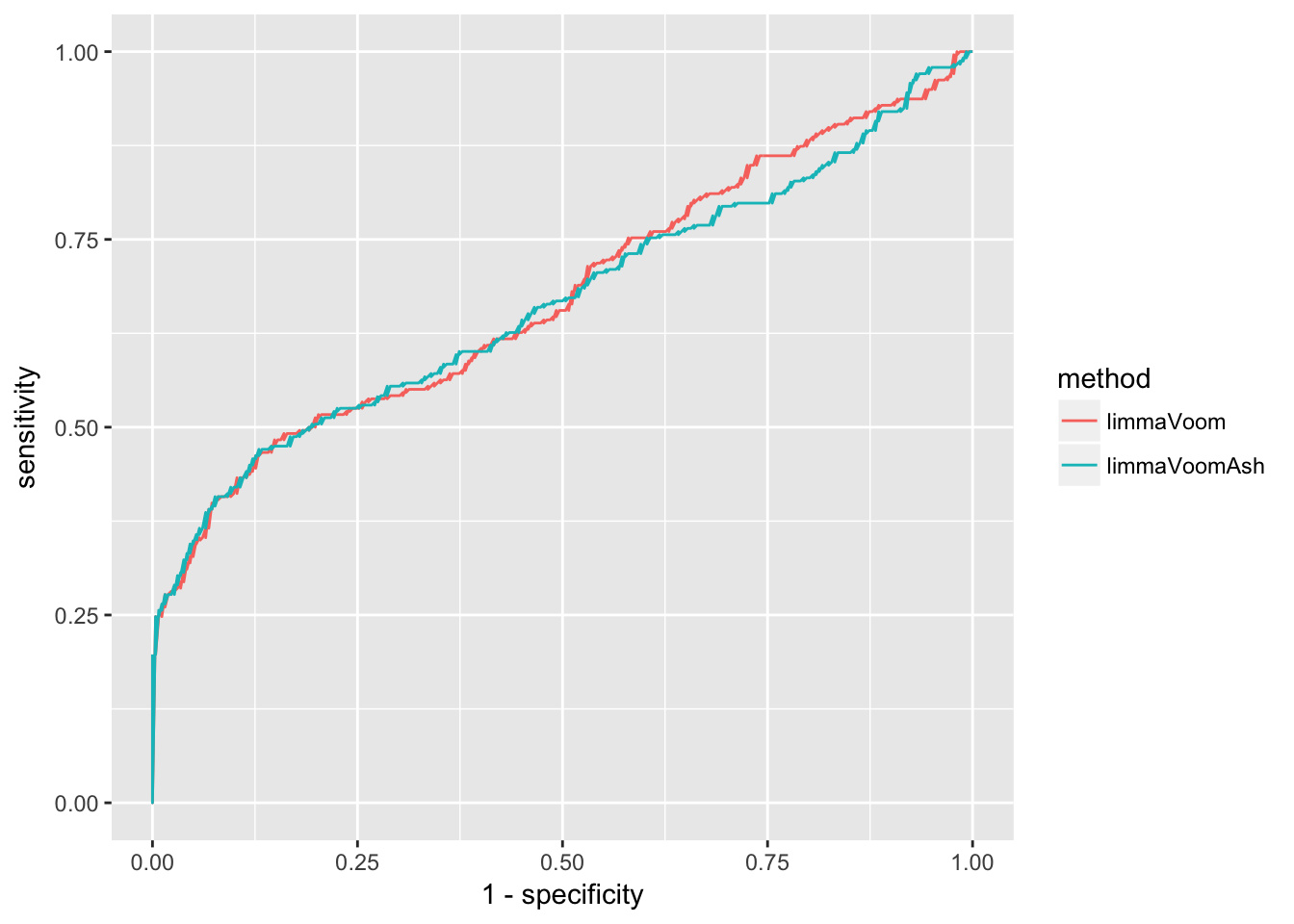 

List the value of true positive rate at false positive rate of .05.

foo <- subset(roc.plot_pROC, sensitivity < .05)
foo[order(foo$sensitivity, decreasing = TRUE), ]

           method sensitivity specificity
489     limmaVoom 0.046218487           1
989  limmaVoomAsh 0.046218487           1
490     limmaVoom 0.042016807           1
990  limmaVoomAsh 0.042016807           1
491     limmaVoom 0.037815126           1
991  limmaVoomAsh 0.037815126           1
492     limmaVoom 0.033613445           1
992  limmaVoomAsh 0.033613445           1
493     limmaVoom 0.029411765           1
993  limmaVoomAsh 0.029411765           1
494     limmaVoom 0.025210084           1
994  limmaVoomAsh 0.025210084           1
495     limmaVoom 0.021008403           1
995  limmaVoomAsh 0.021008403           1
496     limmaVoom 0.016806723           1
996  limmaVoomAsh 0.016806723           1
497     limmaVoom 0.012605042           1
997  limmaVoomAsh 0.012605042           1
498     limmaVoom 0.008403361           1
998  limmaVoomAsh 0.008403361           1
499     limmaVoom 0.004201681           1
999  limmaVoomAsh 0.004201681           1
500     limmaVoom 0.000000000           1
1000 limmaVoomAsh 0.000000000           1