Sample QC
Po-Yuan Tung
Last updated: 2020-01-23
Checks: 7 0
Knit directory: peco-paper/
This reproducible R Markdown analysis was created with workflowr (version 1.6.0). The Checks tab describes the reproducibility checks that were applied when the results were created. The Past versions tab lists the development history.
Great! Since the R Markdown file has been committed to the Git repository, you know the exact version of the code that produced these results.
Great job! The global environment was empty. Objects defined in the global environment can affect the analysis in your R Markdown file in unknown ways. For reproduciblity it’s best to always run the code in an empty environment.
The command set.seed(20190814) was run prior to running the code in the R Markdown file. Setting a seed ensures that any results that rely on randomness, e.g. subsampling or permutations, are reproducible.
Great job! Recording the operating system, R version, and package versions is critical for reproducibility.
Nice! There were no cached chunks for this analysis, so you can be confident that you successfully produced the results during this run.
Great job! Using relative paths to the files within your workflowr project makes it easier to run your code on other machines.
Great! You are using Git for version control. Tracking code development and connecting the code version to the results is critical for reproducibility. The version displayed above was the version of the Git repository at the time these results were generated.
Note that you need to be careful to ensure that all relevant files for the analysis have been committed to Git prior to generating the results (you can use wflow_publish or wflow_git_commit). workflowr only checks the R Markdown file, but you know if there are other scripts or data files that it depends on. Below is the status of the Git repository when the results were generated:
Ignored files:
    Ignored:    .Rhistory
    Ignored:    .Rproj.user/

Untracked files:
    Untracked:  analysis/gene-filtering.Rmd
    Untracked:  analysis/npreg_trendfilter_quantile.Rmd
    Untracked:  analysis/pca-tf.Rmd
    Untracked:  code/fig2_rev.R
    Untracked:  data/fit.quant.rds
    Untracked:  data/intensity.rds
    Untracked:  data/log2cpm.quant.rds

Unstaged changes:
    Modified:   analysis/access_data.Rmd
    Modified:   analysis/index.Rmd
    Modified:   code/fig2.R
Note that any generated files, e.g. HTML, png, CSS, etc., are not included in this status report because it is ok for generated content to have uncommitted changes.
These are the previous versions of the R Markdown and HTML files. If you’ve configured a remote Git repository (see ?wflow_git_remote), click on the hyperlinks in the table below to view them.
| File | Version | Author | Date | Message |
|---|---|---|---|---|
| Rmd | 3f2b8a8 | jhsiao999 | 2020-01-23 | move sampleqc.Rmd and change eset to sce |
| html | 179ec00 | jhsiao999 | 2020-01-23 | Build site. |
| Rmd | 0f6f533 | jhsiao999 | 2020-01-23 | copy and update eset to sce in sampleqc.Rmd |
Setup
library("cowplot")
library("dplyr")
library("edgeR")
library("ggplot2")
library("MASS")
library("tibble")
library("SingleCellExperiment")
theme_set(cowplot::theme_cowplot())

# The palette with grey:
cbPalette <- c("#999999", "#E69F00", "#56B4E9", "#009E73", "#F0E442", "#0072B2", "#D55E00", "#CC79A7")
indi_palette <- c("tomato4", "chocolate1", "rosybrown", "purple4", "plum3", "slateblue")
sce_raw <- readRDS("data/sce-raw.rds")
anno <- data.frame(colData(sce_raw))Total mapped reads
Note: Using the 20 % cutoff of samples with no cells excludes all the samples
## calculate the cut-off
cut_off_reads <- quantile(anno[anno$cell_number == 0,"mapped"], 0.82)

cut_off_reads
82%
1309921 anno$cut_off_reads <- anno$mapped > cut_off_reads
## numbers of cells
sum(anno[anno$cell_number == 1, "mapped"] > cut_off_reads)[1] 978sum(anno[anno$cell_number == 1, "mapped"] <= cut_off_reads)[1] 349## density plots
plot_reads <- ggplot(anno[anno$cell_number == 0 |
anno$cell_number == 1 , ],
aes(x = mapped, fill = as.factor(cell_number))) +
geom_density(alpha = 0.5) +
geom_vline(xintercept = cut_off_reads, colour="grey", linetype = "longdash") +
labs(x = "Total mapped reads", title = "Number of total mapped reads", fill = "Cell number")
plot_reads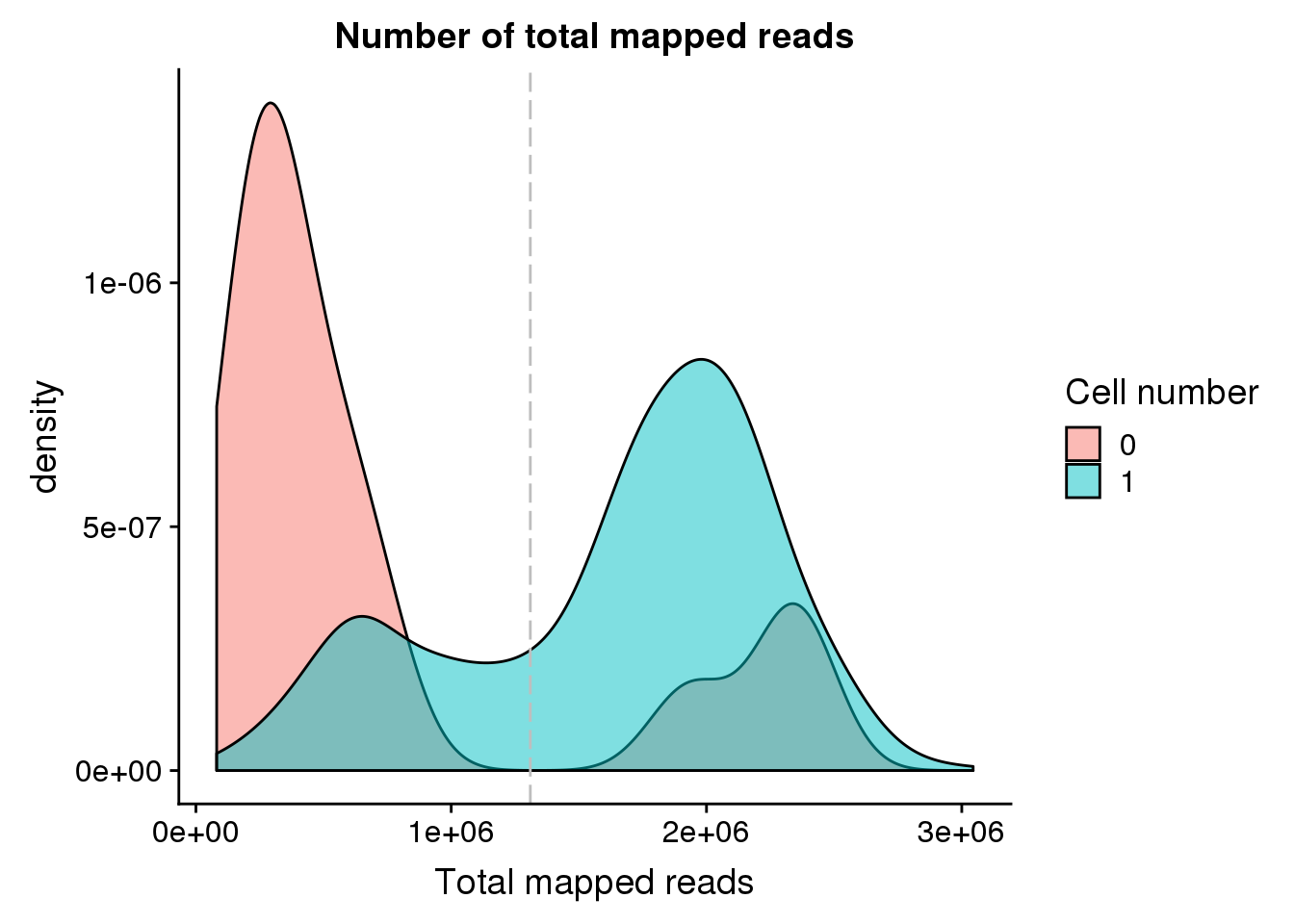
| Version | Author | Date |
|---|---|---|
| 179ec00 | jhsiao999 | 2020-01-23 |
Unmapped ratios
Note: Using the 40 % cutoff of samples with no cells excludes all the samples
## calculate unmapped ratios
anno$unmapped_ratios <- anno$unmapped/anno$umi

## cut off
cut_off_unmapped <- quantile(anno[anno$cell_number == 0,"unmapped_ratios"], 0.40)

cut_off_unmapped
40%
0.4362152 anno$cut_off_unmapped <- anno$unmapped_ratios < cut_off_unmapped
## numbers of cells
sum(anno[anno$cell_number == 1, "unmapped_ratios"] >= cut_off_unmapped)[1] 221sum(anno[anno$cell_number == 1, "unmapped_ratios"] < cut_off_unmapped)[1] 1106## density plots
plot_unmapped <- ggplot(anno[anno$cell_number == 0 |
anno$cell_number == 1 , ],
aes(x = unmapped_ratios *100, fill = as.factor(cell_number))) +
geom_density(alpha = 0.5) +
geom_vline(xintercept = cut_off_unmapped *100, colour="grey", linetype = "longdash") +
labs(x = "Unmapped reads/ total reads", title = "Unmapped reads percentage")
plot_unmapped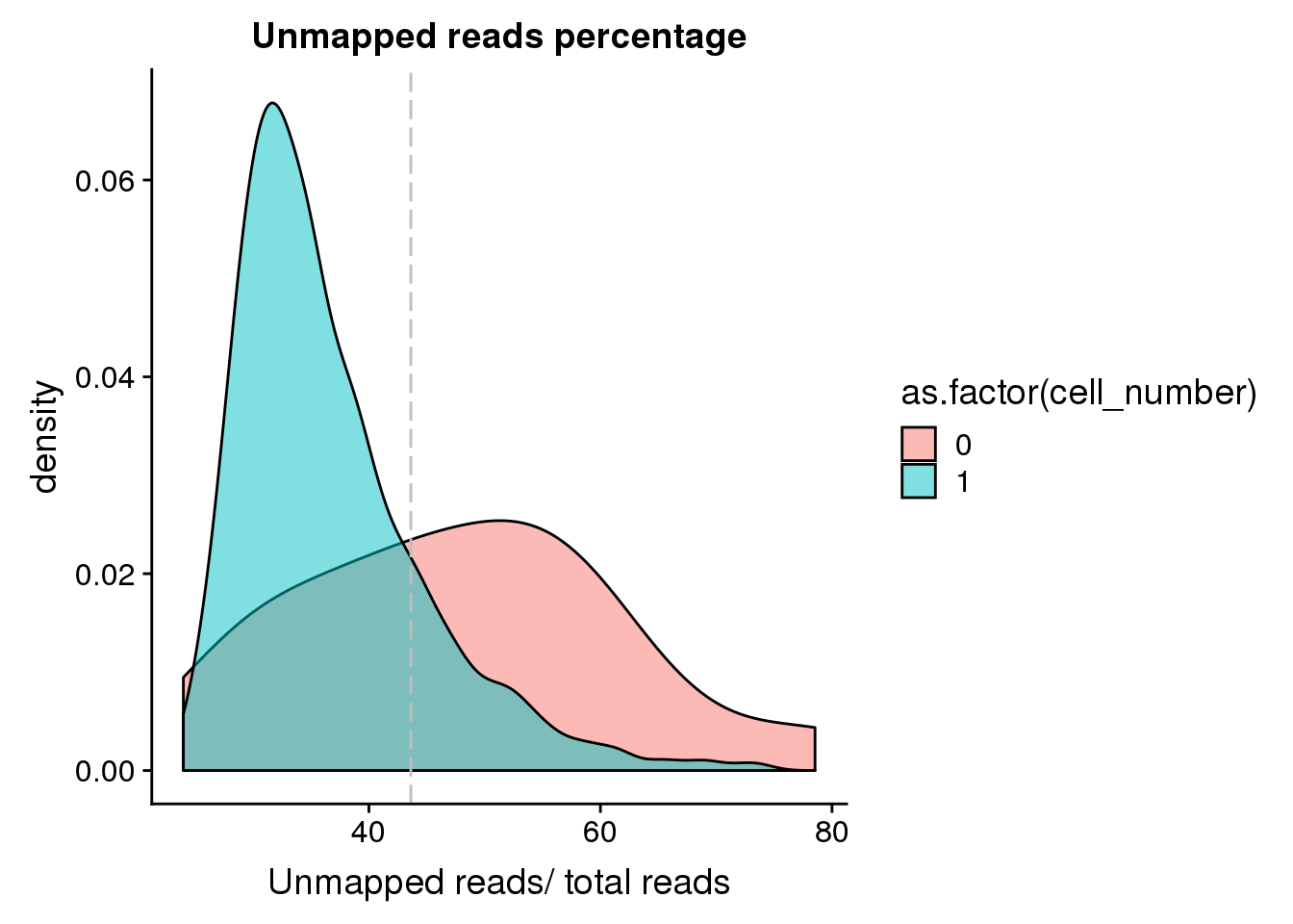
| Version | Author | Date |
|---|---|---|
| 179ec00 | jhsiao999 | 2020-01-23 |
Look at the unmapped percentage per sample by C1 experimnet and by individual.
unmapped_exp <- ggplot(anno, aes(x = as.factor(experiment), y = unmapped_ratios, color = as.factor(experiment))) +
  geom_violin() +
  geom_boxplot(alpha = .01, width = .2, position = position_dodge(width = .9)) +
  labs(x = "C1 chip", y = "Unmapped reads/ total reads",
       title = "Unmapped reads percentage") +
  theme(legend.title = element_blank(),
        axis.text.x = element_text(angle = 45, hjust = 1, vjust = 1))

unmapped_indi <- ggplot(anno, aes(x = chip_id, y = unmapped_ratios, color = as.factor(chip_id))) +
  geom_violin() +
  geom_boxplot(alpha = .01, width = .2, position = position_dodge(width = .9)) +
  scale_color_manual(values = indi_palette) +
  labs(x = "C1 chip", y = "Unmapped reads/ total reads",
       title = "Unmapped reads percentage") +
  theme(legend.title = element_blank(),
        axis.text.x = element_text(angle = 45, hjust = 1, vjust = 1))

plot_grid(unmapped_exp + theme(legend.position = "none"),
          unmapped_indi + theme(legend.position = "none"),
          labels = letters[1:2])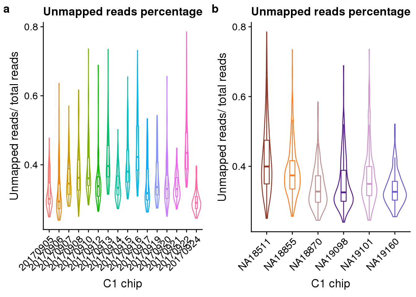
| Version | Author | Date |
|---|---|---|
| 179ec00 | jhsiao999 | 2020-01-23 |
ERCC percentage
## calculate ercc reads percentage
anno$ercc_percentage <- anno$reads_ercc / anno$mapped

## cut off
cut_off_ercc <- quantile(anno[anno$cell_number == 0,"ercc_percentage"], 0.20)

cut_off_ercc
20%
0.179423 anno$cut_off_ercc <- anno$ercc_percentage < cut_off_ercc
## numbers of cells
sum(anno[anno$cell_number == 1, "ercc_percentage"] >= cut_off_ercc)[1] 223sum(anno[anno$cell_number == 1, "ercc_percentage"] < cut_off_ercc)[1] 1104## density plots
plot_ercc <- ggplot(anno[anno$cell_number == 0 |
anno$cell_number == 1 , ],
aes(x = ercc_percentage *100, fill = as.factor(cell_number))) +
geom_density(alpha = 0.5) +
geom_vline(xintercept = cut_off_ercc *100, colour="grey", linetype = "longdash") +
labs(x = "ERCC reads / total mapped reads", title = "ERCC reads percentage")
plot_ercc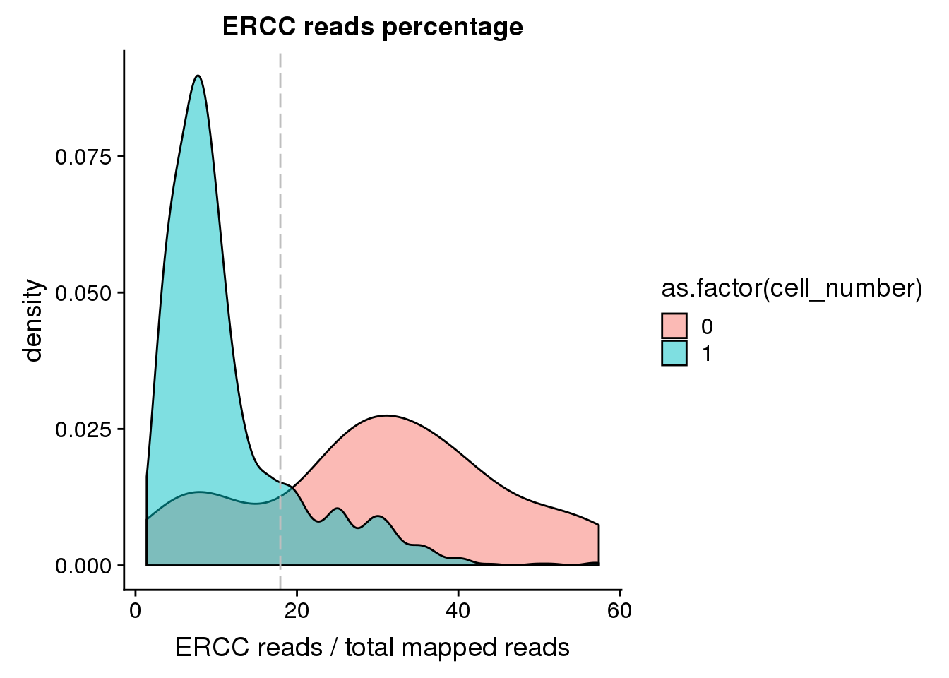
| Version | Author | Date |
|---|---|---|
| 179ec00 | jhsiao999 | 2020-01-23 |
Look at the ERCC spike-in percentage per sample by C1 experimnet and by individual.
ercc_exp <- ggplot(anno, aes(x = as.factor(experiment), y = ercc_percentage, color = as.factor(experiment))) +
  geom_violin() +
  geom_boxplot(alpha = .01, width = .2, position = position_dodge(width = .9)) +
  labs(x = "C1 chip", y = "ERCC percentage",
       title = "ERCC percentage per sample") +
  theme(legend.title = element_blank(),
        axis.text.x = element_text(angle = 45, hjust = 1, vjust = 1))

ercc_indi <- ggplot(anno, aes(x = chip_id, y = ercc_percentage, color = as.factor(chip_id))) +
  geom_violin() +
  geom_boxplot(alpha = .01, width = .2, position = position_dodge(width = .9)) +
  scale_colour_manual(values = indi_palette) +
  labs(x = "C1 chip", y = "ERCC percentage",
       title = "ERCC percentage per sample") +
  theme(legend.title = element_blank(),
        axis.text.x = element_text(angle = 45, hjust = 1, vjust = 1))

plot_grid(ercc_exp + theme(legend.position = "none"),
          ercc_indi + theme(legend.position = "none"),
          labels = letters[1:2])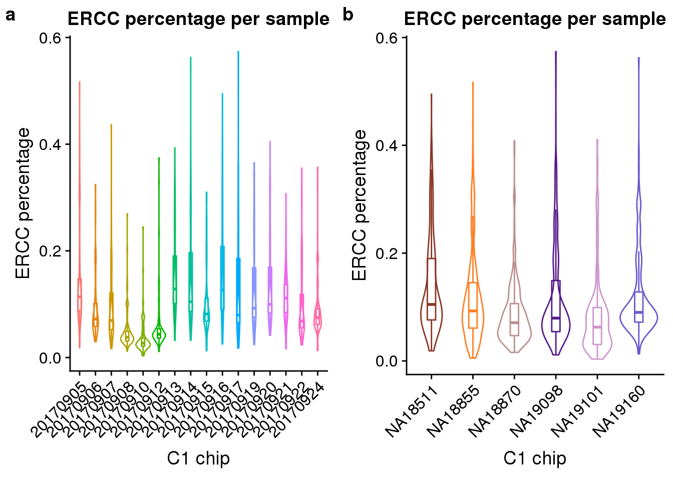
| Version | Author | Date |
|---|---|---|
| 179ec00 | jhsiao999 | 2020-01-23 |
Number of genes detected
## cut off
cut_off_genes <- quantile(anno[anno$cell_number == 0,"detect_hs"], 0.80)

cut_off_genes
80%
6291.8 anno$cut_off_genes <- anno$detect_hs > cut_off_genes
## numbers of cells
sum(anno[anno$cell_number == 1, "detect_hs"] > cut_off_genes)[1] 1040sum(anno[anno$cell_number == 1, "detect_hs"] <= cut_off_genes)[1] 287## density plots
plot_gene <- ggplot(anno[anno$cell_number == 0 |
anno$cell_number == 1 , ],
aes(x = detect_hs, fill = as.factor(cell_number))) +
geom_density(alpha = 0.5) +
geom_vline(xintercept = cut_off_genes, colour="grey", linetype = "longdash") +
labs(x = "Gene numbers", title = "Numbers of detected genes")
plot_gene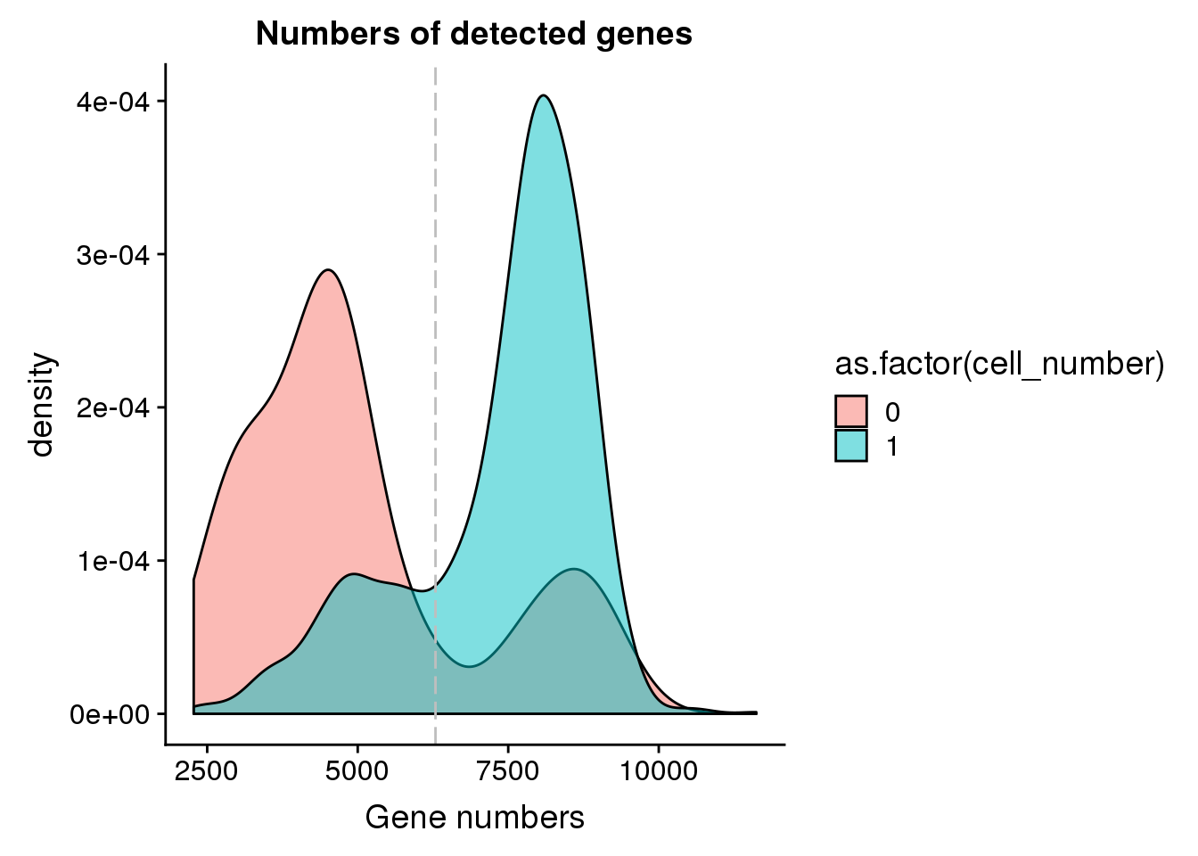
| Version | Author | Date |
|---|---|---|
| 179ec00 | jhsiao999 | 2020-01-23 |
number_exp <- ggplot(anno, aes(x = as.factor(experiment), y = detect_hs, color = as.factor(experiment))) +
  geom_violin() +
  geom_boxplot(alpha = .01, width = .2, position = position_dodge(width = .9)) +
  labs(x = "C1 chip", y = "Number of genes detected",
       title = "Number of genes per sample") +
  theme(legend.title = element_blank(),
        axis.text.x = element_text(angle = 45, hjust = 1, vjust = 1))

number_indi <- ggplot(anno, aes(x = chip_id, y = detect_hs, color = as.factor(chip_id))) +
  geom_violin() +
  geom_boxplot(alpha = .01, width = .2, position = position_dodge(width = .9)) +
  scale_colour_manual(values = indi_palette) +
  labs(x = "C1 chip", y = "Number of genes detected",
       title = "Number of genes per sample") +
  theme(legend.title = element_blank(),
        axis.text.x = element_text(angle = 45, hjust = 1, vjust = 1))

plot_grid(number_exp + theme(legend.position = "none"),
          number_indi + theme(legend.position = "none"),
          labels = letters[1:2])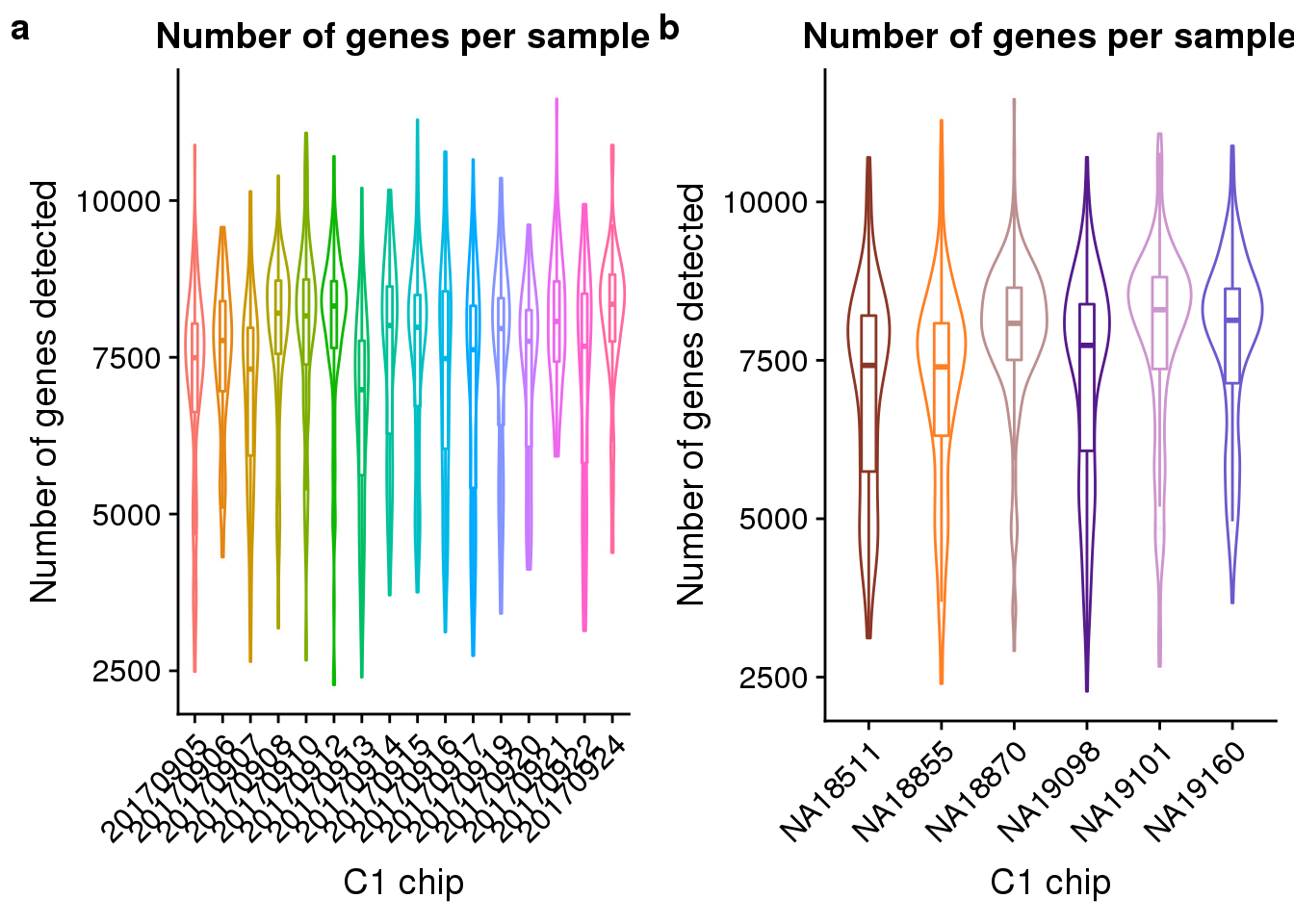
| Version | Author | Date |
|---|---|---|
| 179ec00 | jhsiao999 | 2020-01-23 |
FUCCI transgene
## plot molecule number of egfp and mCherry
egfp_mol <- ggplot(anno[anno$cell_number == 0 |
            anno$cell_number == 1 , ],
       aes(x = mol_egfp, fill = as.factor(cell_number))) +
       geom_density(alpha = 0.5) +
       labs(x = "EGFP molecule numbers", title = "Numbers of EGFP molecules")

mcherry_mol <- ggplot(anno[anno$cell_number == 0 |
            anno$cell_number == 1 , ],
       aes(x = mol_mcherry, fill = as.factor(cell_number))) +
       geom_density(alpha = 0.5) +
       labs(x = "mCherry molecule numbers", title = "Numbers of mCherry molecules")

plot_grid(egfp_mol + theme(legend.position = c(.5,.9)),
          mcherry_mol + theme(legend.position = "none"),
          labels = letters[1:2])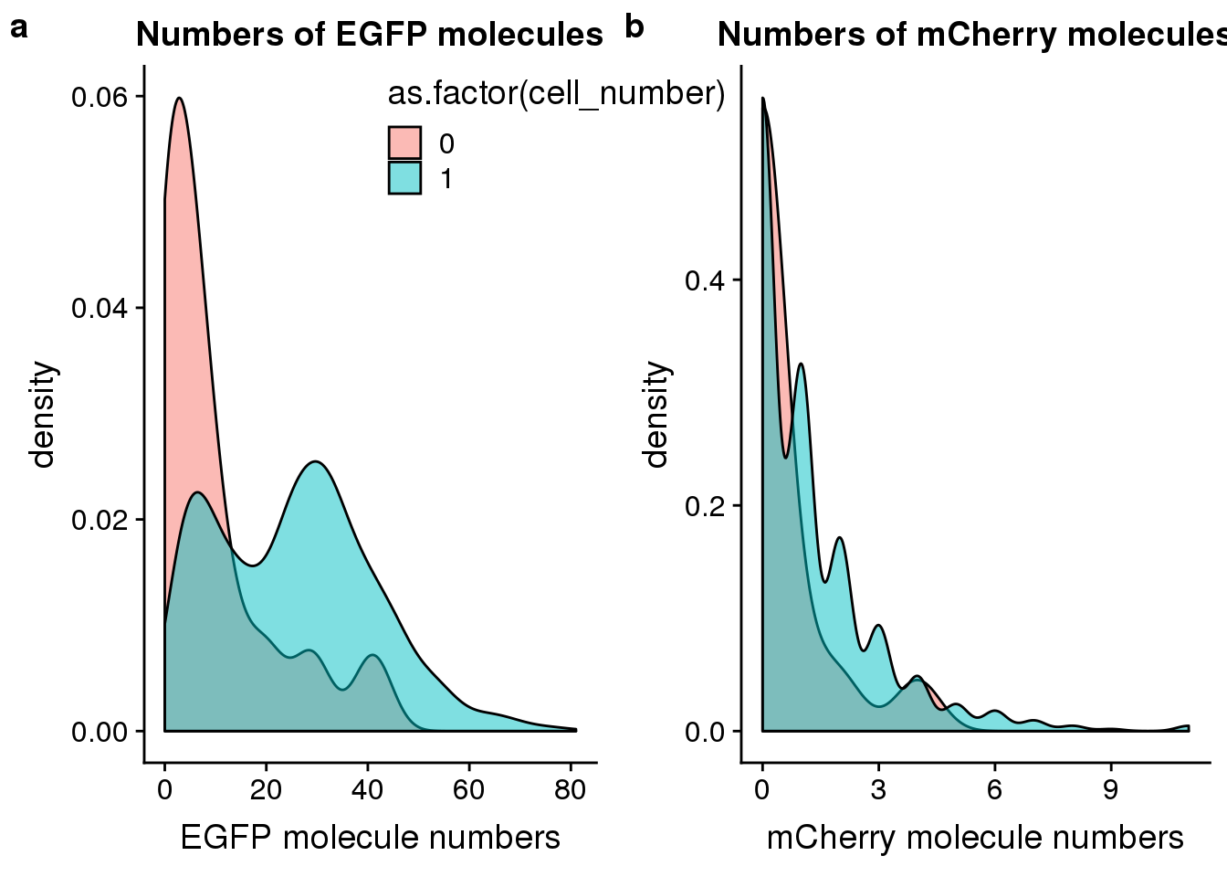
| Version | Author | Date |
|---|---|---|
| 179ec00 | jhsiao999 | 2020-01-23 |
Linear Discriminat Analysis
Total molecule vs concentration
## create 3 groups according to cell number
group_3 <- rep("two",dim(anno)[1])
         group_3[grep("0", anno$cell_number)] <- "no"
         group_3[grep("1", anno$cell_number)] <- "one"

## create data frame
data <- anno %>% dplyr::select(experiment:concentration, mapped, molecules)
data <- data.frame(data, group = group_3)

## perform lda
data_lda <- lda(group ~ concentration + molecules, data = data)
data_lda_p <- predict(data_lda, newdata = data[,c("concentration", "molecules")])$class

## determine how well the model fix
table(data_lda_p, data[, "group"])
data_lda_p   no  one  two
       no     0    0    0
       one   16 1317  147
       two    0   11   45
data$data_lda_p <- data_lda_p
## identify the outlier
outliers_lda <- data %>% rownames_to_column("sample_id") %>% filter(cell_number == 1, data_lda_p == "two")
outliers_lda sample_id experiment well cell_number concentration mapped
1 20170910-H09 20170910 H09 1 1.6540139 3013565
2 20170914-B04 20170914 B04 1 1.3324572 2284753
3 20170914-C04 20170914 C04 1 1.2389752 2489489
4 20170916-A08 20170916 A08 1 0.4900687 2276922
5 20170921-A12 20170921 A12 1 1.7967793 1868421
6 20170921-C01 20170921 C01 1 1.4171401 1543484
7 20170921-D04 20170921 D04 1 1.0853582 1753336
8 20170921-H09 20170921 H09 1 0.5802048 1541776
9 20170924-A04 20170924 A04 1 0.9856825 1414428
10 20170924-E01 20170924 E01 1 0.4581647 1817801
11 20170924-E03 20170924 E03 1 0.4484874 1924140
molecules group data_lda_p
1 281516 one two
2 190473 one two
3 205586 one two
4 169065 one two
5 205868 one two
6 202756 one two
7 255148 one two
8 415411 one two
9 253058 one two
10 187137 one two
11 346383 one two## create filter
anno$molecule_outlier <- row.names(anno) %in% outliers_lda$sample_id
## plot before and after
plot_before <- ggplot(data, aes(x = concentration, y = molecules / 10^3,
color = as.factor(group))) +
geom_text(aes(label = cell_number, alpha = 0.5)) +
labs(x = "Concentration", y = "Gene molecules (thousands)", title = "Before") +
scale_color_brewer(palette = "Dark2") +
theme(legend.position = "none")
plot_after <- ggplot(data, aes(x = concentration, y = molecules / 10^3,
color = as.factor(data_lda_p))) +
geom_text(aes(label = cell_number, alpha = 0.5)) +
labs(x = "Concentration", y = "Gene molecules (thousands)", title = "After") +
scale_color_brewer(palette = "Dark2") +
theme(legend.position = "none")
plot_grid(plot_before + theme(legend.position=c(.8,.85)),
plot_after + theme(legend.position = "none"),
labels = LETTERS[1:2])
| Version | Author | Date |
|---|---|---|
| 179ec00 | jhsiao999 | 2020-01-23 |
Reads to molecule conversion
## calculate convertion
anno$ercc_conversion <- anno$mol_ercc / anno$reads_ercc

anno$conversion <- anno$mol_hs / anno$reads_hs

## try lda
data$conversion <- anno$conversion
data$ercc_conversion <- anno$ercc_conversion

data_ercc_lda <- lda(group ~ ercc_conversion + conversion, data = data)

data_ercc_lda_p <- predict(data_ercc_lda,  newdata = data[,c("ercc_conversion", "conversion")])$class

## determine how well the model fix
table(data_ercc_lda_p, data[, "group"])
data_ercc_lda_p   no  one  two
            no     5   20    0
            one   11 1303  166
            two    0    5   26
data$data_ercc_lda_p <- data_ercc_lda_p
## identify the outlier
outliers_conversion <- data %>% rownames_to_column("sample_id") %>% filter(cell_number == 1, data_ercc_lda_p == "two")
outliers_conversion sample_id experiment well cell_number concentration mapped molecules
1 20170908-C07 20170908 C07 1 2.6936993 850577 95163
2 20170920-A10 20170920 A10 1 0.1369852 81371 28680
3 20170921-H09 20170921 H09 1 0.5802048 1541776 415411
4 20170924-A04 20170924 A04 1 0.9856825 1414428 253058
5 20170924-E03 20170924 E03 1 0.4484874 1924140 346383
group data_lda_p conversion ercc_conversion data_ercc_lda_p
1 one one 0.1126820 0.08186312 two
2 one one 0.3585794 0.24727354 two
3 one two 0.2716902 0.13085675 two
4 one two 0.1809263 0.09389137 two
5 one two 0.1813526 0.10260360 two## create filter
anno$conversion_outlier <- row.names(anno) %in% outliers_conversion$sample_id
## plot before and after
plot_ercc_before <- ggplot(data, aes(x = ercc_conversion, y = conversion,
color = as.factor(group))) +
geom_text(aes(label = cell_number, alpha = 0.5)) +
labs(x = "Convertion of ERCC spike-ins", y = "Conversion of genes", title = "Before") +
scale_color_brewer(palette = "Dark2") +
theme(legend.position = "none")
plot_ercc_after <- ggplot(data, aes(x = ercc_conversion, y = conversion,
color = as.factor(data_ercc_lda_p))) +
geom_text(aes(label = cell_number, alpha = 0.5)) +
labs(x = "Convertion of ERCC spike-ins", y = "Conversion of genes", title = "After") +
scale_color_brewer(palette = "Dark2") +
theme(legend.position = "none")
plot_grid(plot_ercc_before,
plot_ercc_after,
labels = LETTERS[3:4])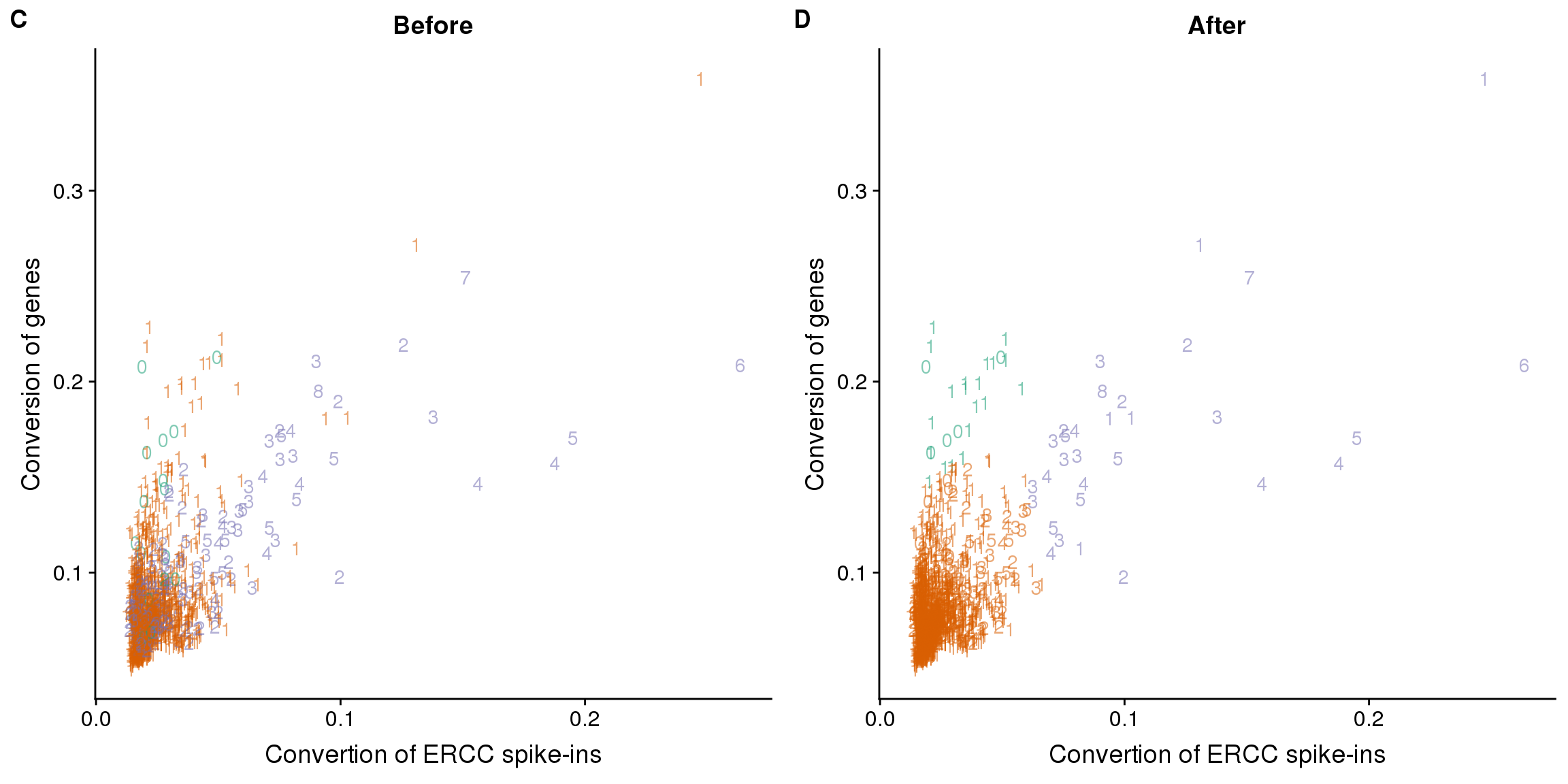
| Version | Author | Date |
|---|---|---|
| 179ec00 | jhsiao999 | 2020-01-23 |
PCA
## look at human genes
sce_hs <- sce_raw[rowData(sce_raw)$source == "H. sapiens", ]
head(colData(sce_hs))
DataFrame with 6 rows and 44 columns
experiment well cell_number concentration ERCC
<integer> <character> <integer> <numeric> <character>
20170905-A01 20170905 A01 1 1.726404375 50x dilution
20170905-A02 20170905 A02 1 1.445692561 50x dilution
20170905-A03 20170905 A03 1 1.889617025 50x dilution
20170905-A04 20170905 A04 1 0.47537227 50x dilution
20170905-A05 20170905 A05 1 0.559682703 50x dilution
20170905-A06 20170905 A06 1 2.135351839 50x dilution
individual.1 individual.2 image_individual image_label
<character> <character> <character> <integer>
20170905-A01 NA18855 NA18870 18870_18855 3
20170905-A02 NA18855 NA18870 18870_18855 2
20170905-A03 NA18855 NA18870 18870_18855 1
20170905-A04 NA18855 NA18870 18870_18855 49
20170905-A05 NA18855 NA18870 18870_18855 50
20170905-A06 NA18855 NA18870 18870_18855 51
raw umi mapped unmapped reads_ercc reads_hs
<integer> <integer> <integer> <integer> <integer> <integer>
20170905-A01 5746265 3709414 2597589 1111825 161686 2435427
20170905-A02 3997709 2642317 1799823 842494 253670 1545769
20170905-A03 4765829 3301270 2274259 1027011 261145 2011561
20170905-A04 1926305 1286653 806647 480006 247028 559614
20170905-A05 2626155 1740464 1036933 703531 247831 788955
20170905-A06 5249443 3662342 2631138 1031204 210518 2419498
reads_egfp reads_mcherry molecules mol_ercc mol_hs
<integer> <integer> <integer> <integer> <integer>
20170905-A01 475 1 158546 3692 154830
20170905-A02 379 5 88552 3648 84887
20170905-A03 1550 3 107984 3820 104119
20170905-A04 5 0 44772 3505 41262
20170905-A05 145 2 64926 3505 61413
20170905-A06 1118 4 134989 3664 131293
mol_egfp mol_mcherry detect_ercc detect_hs chip_id
<integer> <integer> <numeric> <numeric> <character>
20170905-A01 23 1 41 9018 NA18870
20170905-A02 12 5 45 6848 NA18870
20170905-A03 44 1 44 7228 NA18855
20170905-A04 5 0 43 3653 NA18870
20170905-A05 6 2 44 4704 NA18870
20170905-A06 31 1 43 8198 NA18870
chipmix freemix snps reads avg_dp min_dp
<numeric> <numeric> <integer> <integer> <numeric> <integer>
20170905-A01 0.16693 0.05395 311848 9356 0.03 1
20170905-A02 0.26917 0.13813 311848 4678 0.02 1
20170905-A03 0.36964 0.07778 311848 6201 0.02 1
20170905-A04 0.5132 0.2615 311848 1356 0 1
20170905-A05 0.54431 0.21419 311848 1906 0.01 1
20170905-A06 0.22935 0.08126 311848 7929 0.03 1
snps_w_min valid_id cut_off_reads unmapped_ratios
<integer> <logical> <logical> <numeric>
20170905-A01 3961 TRUE TRUE 0.299730631307263
20170905-A02 2201 TRUE TRUE 0.318846678880694
20170905-A03 2550 TRUE TRUE 0.311095729825188
20170905-A04 857 TRUE FALSE 0.373065620645193
20170905-A05 1139 TRUE FALSE 0.404220368821188
20170905-A06 3190 TRUE TRUE 0.281569553034643
cut_off_unmapped ercc_percentage cut_off_ercc
<logical> <numeric> <logical>
20170905-A01 TRUE 0.0622446430131942 TRUE
20170905-A02 TRUE 0.140941637038753 TRUE
20170905-A03 TRUE 0.114826411591644 TRUE
20170905-A04 TRUE 0.306240524045834 FALSE
20170905-A05 TRUE 0.239003870066822 FALSE
20170905-A06 TRUE 0.0800102465169064 TRUE
cut_off_genes ercc_conversion conversion
<logical> <numeric> <numeric>
20170905-A01 TRUE 0.0228343826923791 0.0635740672990814
20170905-A02 TRUE 0.014380888555998 0.0549157086214046
20170905-A03 TRUE 0.0146278887208256 0.0517602995882302
20170905-A04 FALSE 0.0141886749680198 0.0737329659372353
20170905-A05 FALSE 0.0141427020832745 0.0778409414985646
20170905-A06 TRUE 0.0174046874851557 0.0542645623182991
conversion_outlier molecule_outlier filter_all
<logical> <logical> <logical>
20170905-A01 FALSE FALSE TRUE
20170905-A02 FALSE FALSE TRUE
20170905-A03 FALSE FALSE TRUE
20170905-A04 FALSE FALSE FALSE
20170905-A05 FALSE FALSE FALSE
20170905-A06 FALSE FALSE TRUE## remove genes of all 0s
sce_hs_clean <- sce_hs[rowSums(assay(sce_hs)) != 0, ]
dim(sce_hs_clean)[1] 19348 1536## convert to log2 cpm
mol_hs_cpm <- edgeR::cpm(assay(sce_hs_clean), log = TRUE)
mol_hs_cpm_means <- rowMeans(mol_hs_cpm)
summary(mol_hs_cpm_means) Min. 1st Qu. Median Mean 3rd Qu. Max.
5.412 5.431 5.634 5.987 6.210 13.007 mol_hs_cpm <- mol_hs_cpm[mol_hs_cpm_means > median(mol_hs_cpm_means), ]
dim(mol_hs_cpm)[1] 9674 1536## pca of genes with reasonable expression levels
source("code/utility.R")
pca_hs <- run_pca(mol_hs_cpm)
plot_pca_id <- plot_pca(pca_hs$PCs, pcx = 1, pcy = 2, explained = pca_hs$explained,
metadata = data.frame(colData(sce_hs_clean)), color = "chip_id")
plot_pca_id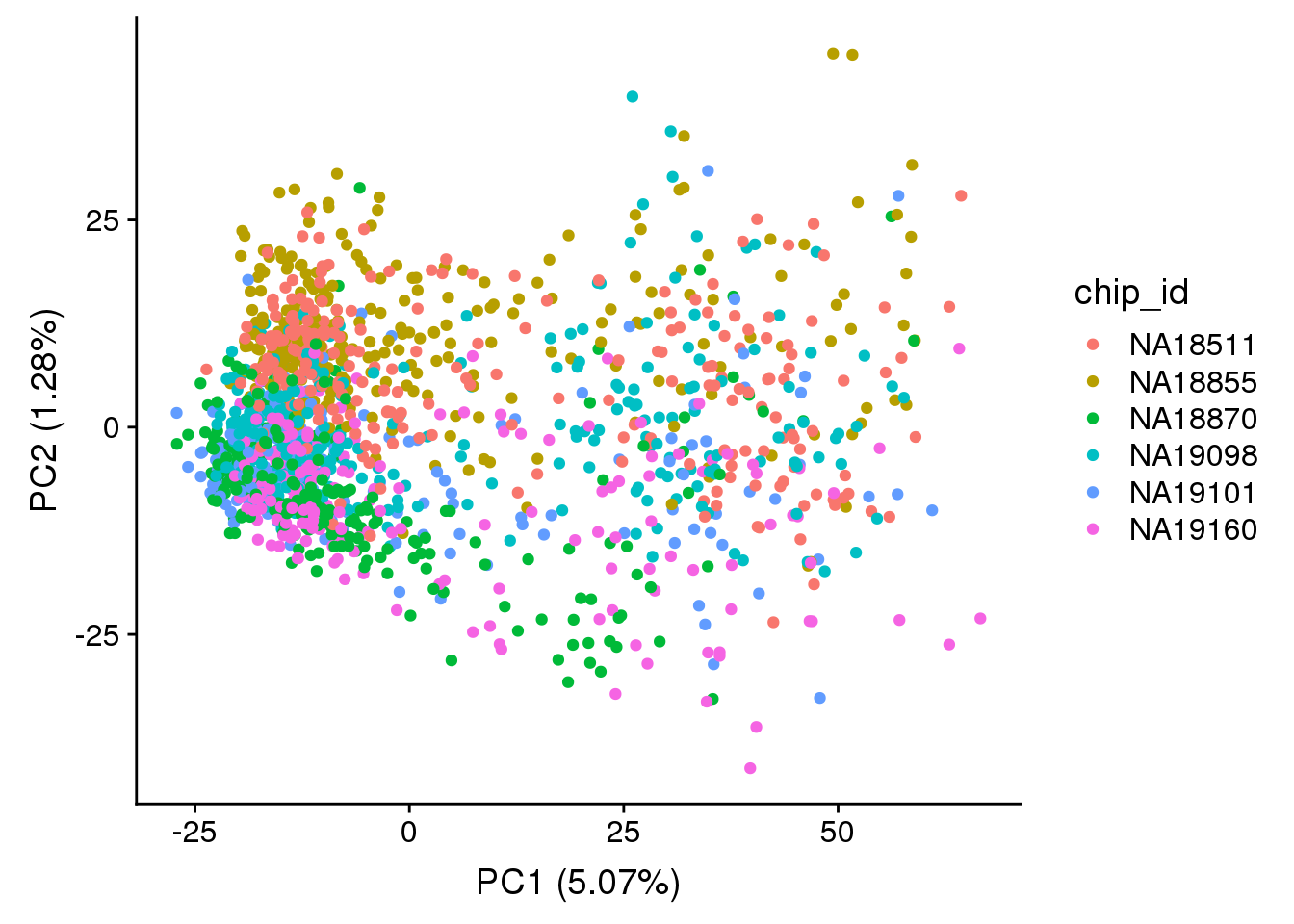
| Version | Author | Date |
|---|---|---|
| 179ec00 | jhsiao999 | 2020-01-23 |
Filter
Final list
## all filter
anno$filter_all <- anno$cell_number == 1 &
                   anno$mol_egfp > 0 &
                   anno$valid_id &
                   anno$cut_off_reads &
                   anno$cut_off_unmapped &
                   anno$cut_off_ercc &
                   anno$cut_off_genes &
                   anno$molecule_outlier == "FALSE" &
                   anno$conversion_outlier == "FALSE"
sort(table(anno[anno$filter_all, "chip_id"]))
NA18511 NA19160 NA19101 NA18855 NA19098 NA18870
    104     123     124     171     187     214
table(anno[anno$filter_all, c("experiment","chip_id")]) chip_id
experiment NA18511 NA18855 NA18870 NA19098 NA19101 NA19160
20170905 0 37 32 0 0 0
20170906 0 0 0 41 22 0
20170907 0 29 0 23 0 0
20170908 0 0 32 0 31 0
20170910 0 30 0 0 24 0
20170912 0 0 42 37 0 0
20170913 0 41 0 0 0 9
20170914 0 0 0 0 24 34
20170915 24 34 0 0 0 0
20170916 13 0 0 0 23 0
20170917 0 0 0 40 0 12
20170919 11 0 0 46 0 0
20170920 39 0 0 0 0 18
20170921 0 0 45 0 0 22
20170922 17 0 25 0 0 0
20170924 0 0 38 0 0 28Plots
genes_unmapped <-  ggplot(anno,
                   aes(x = detect_hs, y = unmapped_ratios * 100,
                       col = as.factor(chip_id),
                       label = as.character(cell_number),
                       height = 600, width = 2000)) +
                   scale_colour_manual(values = indi_palette) +
                   geom_text(fontface = 3, alpha = 0.5) +
                   geom_vline(xintercept = cut_off_genes,
                              colour="grey", linetype = "longdash") +
                   geom_hline(yintercept = cut_off_unmapped * 100,
                              colour="grey", linetype = "longdash") +
                   labs(x = "Number of detected genes / sample",
                        y = "Percentage of unmapped reads (%)")

genes_spike <- ggplot(anno,
               aes(x = detect_hs, y = ercc_percentage * 100,
                   col = as.factor(chip_id),
                   label = as.character(cell_number),
                   height = 600, width = 2000)) +
               scale_colour_manual(values = indi_palette) +
               scale_shape_manual(values=c(1:10)) +
               geom_text(fontface = 3, alpha = 0.5) +
               geom_vline(xintercept = cut_off_genes,
                          colour="grey", linetype = "longdash") +
               geom_hline(yintercept = cut_off_ercc * 100,
                          colour="grey", linetype = "longdash") +
               labs(x = "Number of detected genes / samlpe",
                    y = "Percentage of ERCC spike-in reads (%)")

reads_unmapped_num <-  ggplot(anno,
                       aes(x = mapped, y = unmapped_ratios * 100,
                           col = as.factor(experiment),
                           label = as.character(cell_number),
                           height = 600, width = 2000)) +
                       geom_text(fontface = 3, alpha = 0.5) +
                       geom_vline(xintercept = cut_off_reads,
                                  colour="grey", linetype = "longdash") +
                       geom_hline(yintercept = cut_off_unmapped * 100,
                                  colour="grey", linetype = "longdash") +
                       labs(x = "Total mapped reads / sample",
                            y = "Percentage of unmapped reads (%)")

reads_spike_num <- ggplot(anno,
                   aes(x = mapped, y = ercc_percentage * 100,
                       col = as.factor(experiment),
                       label = as.character(cell_number),
                       height = 600, width = 2000)) +
                   geom_text(fontface = 3, alpha = 0.5) +
                   geom_vline(xintercept = cut_off_reads,
                              colour="grey", linetype = "longdash") +
                   geom_hline(yintercept = cut_off_ercc * 100,
                              colour="grey", linetype = "longdash") +
                   labs(x = "Total mapped reads / sample",
                        y = "Percentage of ERCC spike-in reads (%)")

plot_grid(genes_unmapped + theme(legend.position = c(.7,.9)),
          genes_spike + theme(legend.position = "none"),
          labels = letters[1:2])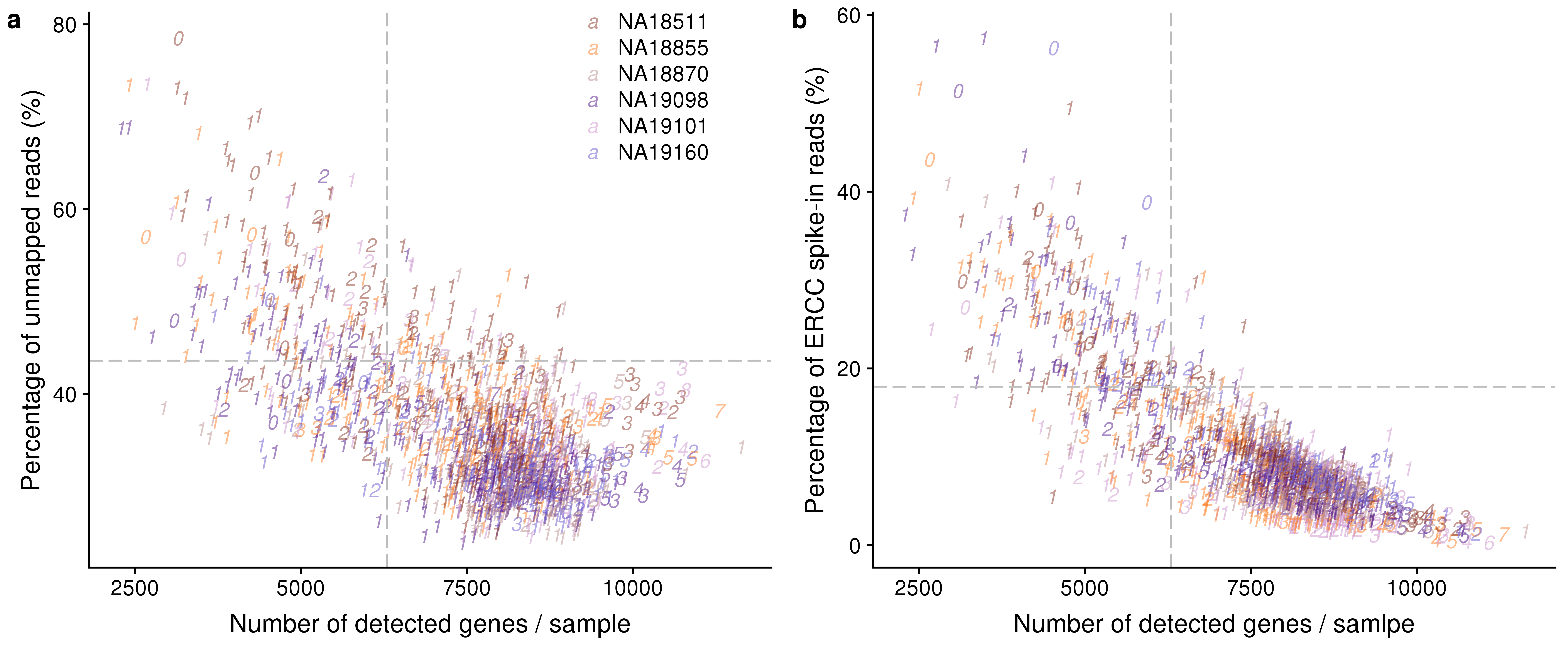
| Version | Author | Date |
|---|---|---|
| 179ec00 | jhsiao999 | 2020-01-23 |
plot_grid(reads_unmapped_num + theme(legend.position = c(.7,.9)),
          reads_spike_num + theme(legend.position = "none"),
          labels = letters[3:4])
| Version | Author | Date |
|---|---|---|
| 179ec00 | jhsiao999 | 2020-01-23 |
ggplot(anno, aes(x = mol_hs, y = detect_hs,
                   col = as.factor(chip_id),
                   height = 600, width = 2000)) +
               scale_colour_manual(values = indi_palette) +
               scale_shape_manual(values=c(1:10)) +
               geom_point(alpha = 0.6) +
               labs(col = "Individual") +
               theme(legend.position = c(.7,.5)) +
               labs(x = "Total molecule counts / samlpe",
y = "Number of detected genes / sample") 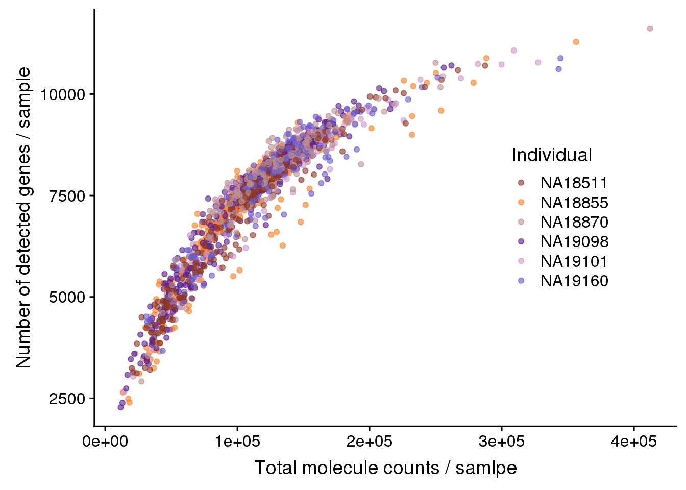
| Version | Author | Date |
|---|---|---|
| 179ec00 | jhsiao999 | 2020-01-23 |
Session information
R version 3.5.1 (2018-07-02)
Platform: x86_64-pc-linux-gnu (64-bit)
Running under: Scientific Linux 7.4 (Nitrogen)

Matrix products: default
BLAS/LAPACK: /software/openblas-0.2.19-el7-x86_64/lib/libopenblas_haswellp-r0.2.19.so

locale:
 [1] LC_CTYPE=en_US.UTF-8       LC_NUMERIC=C
 [3] LC_TIME=en_US.UTF-8        LC_COLLATE=en_US.UTF-8
 [5] LC_MONETARY=en_US.UTF-8    LC_MESSAGES=en_US.UTF-8
 [7] LC_PAPER=en_US.UTF-8       LC_NAME=C
 [9] LC_ADDRESS=C               LC_TELEPHONE=C
[11] LC_MEASUREMENT=en_US.UTF-8 LC_IDENTIFICATION=C

attached base packages:
[1] parallel  stats4    stats     graphics  grDevices utils     datasets
[8] methods   base

other attached packages:
 [1] testit_0.9                  SingleCellExperiment_1.4.1
 [3] SummarizedExperiment_1.12.0 DelayedArray_0.8.0
 [5] BiocParallel_1.16.0         matrixStats_0.55.0
 [7] Biobase_2.42.0              GenomicRanges_1.34.0
 [9] GenomeInfoDb_1.18.1         IRanges_2.16.0
[11] S4Vectors_0.20.1            BiocGenerics_0.28.0
[13] tibble_2.1.1                MASS_7.3-51.1
[15] edgeR_3.24.0                limma_3.38.3
[17] dplyr_0.8.0.1               cowplot_0.9.4
[19] ggplot2_3.2.1

loaded via a namespace (and not attached):
 [1] tidyselect_0.2.5       locfit_1.5-9.1         purrr_0.3.2
 [4] lattice_0.20-38        colorspace_1.3-2       htmltools_0.3.6
 [7] yaml_2.2.0             rlang_0.4.0            later_0.7.5
[10] pillar_1.3.1           glue_1.3.0             withr_2.1.2
[13] RColorBrewer_1.1-2     GenomeInfoDbData_1.2.0 stringr_1.3.1
[16] zlibbioc_1.28.0        munsell_0.5.0          gtable_0.2.0
[19] workflowr_1.6.0        evaluate_0.12          labeling_0.3
[22] knitr_1.20             httpuv_1.4.5           Rcpp_1.0.3
[25] promises_1.0.1         scales_1.0.0           backports_1.1.2
[28] XVector_0.22.0         fs_1.3.1               digest_0.6.20
[31] stringi_1.2.4          grid_3.5.1             rprojroot_1.3-2
[34] tools_3.5.1            bitops_1.0-6           magrittr_1.5
[37] lazyeval_0.2.1         RCurl_1.95-4.11        crayon_1.3.4
[40] whisker_0.3-2          pkgconfig_2.0.3        Matrix_1.2-17
[43] assertthat_0.2.1       rmarkdown_1.10         R6_2.4.0
[46] git2r_0.26.1           compiler_3.5.1
sessionInfo()R version 3.5.1 (2018-07-02)
Platform: x86_64-pc-linux-gnu (64-bit)
Running under: Scientific Linux 7.4 (Nitrogen)
Matrix products: default
BLAS/LAPACK: /software/openblas-0.2.19-el7-x86_64/lib/libopenblas_haswellp-r0.2.19.so
locale:
[1] LC_CTYPE=en_US.UTF-8 LC_NUMERIC=C
[3] LC_TIME=en_US.UTF-8 LC_COLLATE=en_US.UTF-8
[5] LC_MONETARY=en_US.UTF-8 LC_MESSAGES=en_US.UTF-8
[7] LC_PAPER=en_US.UTF-8 LC_NAME=C
[9] LC_ADDRESS=C LC_TELEPHONE=C
[11] LC_MEASUREMENT=en_US.UTF-8 LC_IDENTIFICATION=C
attached base packages:
[1] parallel stats4 stats graphics grDevices utils datasets
[8] methods base
other attached packages:
[1] testit_0.9 SingleCellExperiment_1.4.1
[3] SummarizedExperiment_1.12.0 DelayedArray_0.8.0
[5] BiocParallel_1.16.0 matrixStats_0.55.0
[7] Biobase_2.42.0 GenomicRanges_1.34.0
[9] GenomeInfoDb_1.18.1 IRanges_2.16.0
[11] S4Vectors_0.20.1 BiocGenerics_0.28.0
[13] tibble_2.1.1 MASS_7.3-51.1
[15] edgeR_3.24.0 limma_3.38.3
[17] dplyr_0.8.0.1 cowplot_0.9.4
[19] ggplot2_3.2.1
loaded via a namespace (and not attached):
[1] tidyselect_0.2.5 locfit_1.5-9.1 purrr_0.3.2
[4] lattice_0.20-38 colorspace_1.3-2 htmltools_0.3.6
[7] yaml_2.2.0 rlang_0.4.0 later_0.7.5
[10] pillar_1.3.1 glue_1.3.0 withr_2.1.2
[13] RColorBrewer_1.1-2 GenomeInfoDbData_1.2.0 stringr_1.3.1
[16] zlibbioc_1.28.0 munsell_0.5.0 gtable_0.2.0
[19] workflowr_1.6.0 evaluate_0.12 labeling_0.3
[22] knitr_1.20 httpuv_1.4.5 Rcpp_1.0.3
[25] promises_1.0.1 scales_1.0.0 backports_1.1.2
[28] XVector_0.22.0 fs_1.3.1 digest_0.6.20
[31] stringi_1.2.4 grid_3.5.1 rprojroot_1.3-2
[34] tools_3.5.1 bitops_1.0-6 magrittr_1.5
[37] lazyeval_0.2.1 RCurl_1.95-4.11 crayon_1.3.4
[40] whisker_0.3-2 pkgconfig_2.0.3 Matrix_1.2-17
[43] assertthat_0.2.1 rmarkdown_1.10 R6_2.4.0
[46] git2r_0.26.1 compiler_3.5.1