Example_time_series_example_comparison
- Compare unadjusted p-values from edge and maSigPro (df= 2)
- Compare unadjusted p-values from edge and maSigPro (df= 5)
- Compare Benjamini-Hotchberg corrected p-values from the two software programs
- Compare the number of genes at FDR 1% and FDR 10% for both software programs
- Compare the number of DE genes
- Compare the p-values and q-values of the genes that were statistically significant in both programs
- Session information
Last updated: 2016-08-16
Code version: e0856a352e494c0de5f1f93226e04753d2aebdca
The goal of this section is to compare the results from edge (df = 2) and maSigPro (df = 2) for the endotoxin data.
# Load libraries

library("Hmisc")
Loading required package: latticeLoading required package: survivalLoading required package: FormulaLoading required package: ggplot2
Attaching package: 'Hmisc'The following objects are masked from 'package:base':
format.pval, round.POSIXt, trunc.POSIXt, unitslibrary("formattable")
# Load data
# p-values from edge
p_value_endo_genes_edge_data <- read.csv("../data/p_value_endo_genes_edge_data.txt", sep="")
# p-values from maSigPro (df = 2)
p_value_maSigPro_df_2 <- read.csv("../data/p_value_maSigPro_df_2.txt", sep="")
# p-values from maSigPro (df = 5)
p_value_maSigPro_df_5 <- read.csv("../data/p_value_maSigPro_df_5.txt", sep="")Compare unadjusted p-values from edge and maSigPro (df= 2)
# Combine the two lists of unadjusted p-values into one data frame
unadjust_p_value <- as.data.frame(cbind(p_value_endo_genes_edge_data, p_value_maSigPro_df_2))
colnames(unadjust_p_value) <- c("Unadjusted p-value in edge (df = 2)", "Unadjusted p-value in maSigPro (df = 2)")

# Find the correlation between the two numbers

rc <- rcorr(as.matrix(unadjust_p_value), type="pearson") # Correlation = 0.3766195 and p = approximately 0

flattenCorrMatrix <- function(cormat, pmat) {
  ut <- upper.tri(cormat)
  data.frame(
    row = rownames(cormat)[row(cormat)[ut]],
    column = rownames(cormat)[col(cormat)[ut]],
    cor  =(cormat)[ut],
    p = pmat[ut]
    )
}

flattenCorrMatrix(rc$r, rc$P)
row
1 Unadjusted p-value in edge (df = 2)
column cor p
1 Unadjusted p-value in maSigPro (df = 2) 0.3658995 0# Compare unadjusted p-values from edge and maSigPro
plot(unadjust_p_value, main = "Unadjusted p-values from edge and maSigPro (Pearson's correlation = 0.377)")
# Make a best fit line (which we can then add to the plot)
abline(lm(unadjust_p_value[,1] ~ unadjust_p_value[,2]))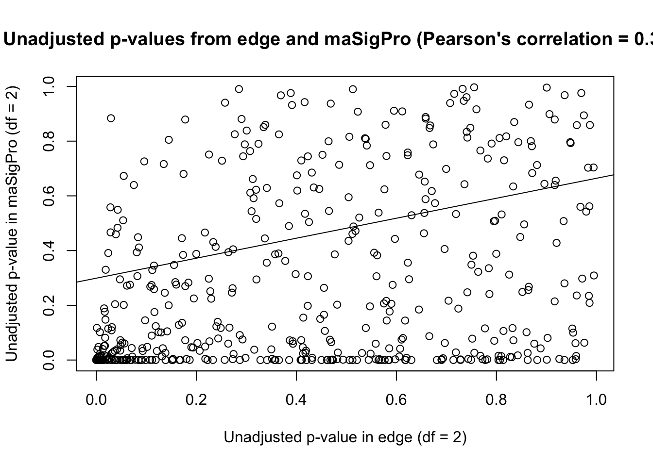
From this plot, it appears that edge is more conservative than maSigPro when df = 2.
Compare unadjusted p-values from edge and maSigPro (df= 5)
# Combine the two lists of unadjusted p-values into one data frame
unadjust_p_value <- as.data.frame(cbind(p_value_endo_genes_edge_data, p_value_maSigPro_df_5))
colnames(unadjust_p_value) <- c("Unadjusted p-values in edge (df = 2)", "Unadjusted p-values in maSigPro (df = 5)")

# Find the correlation between the two numbers

rc <- rcorr(as.matrix(unadjust_p_value), type="pearson") # Correlation = 0.3235 and p = 1.203482e-13

flattenCorrMatrix(rc$r, rc$P)
row
1 Unadjusted p-values in edge (df = 2)
column cor p
1 Unadjusted p-values in maSigPro (df = 5) 0.3095199 1.459277e-12# Compare unadjusted p-values from edge and maSigPro
plot(unadjust_p_value, main = "Unadjusted p-values from edge and maSigPro (Pearson's correlation = 0.324)")
# Make a best fit line (which we can then add to the plot)
abline(lm(unadjust_p_value[,1] ~ unadjust_p_value[,2]))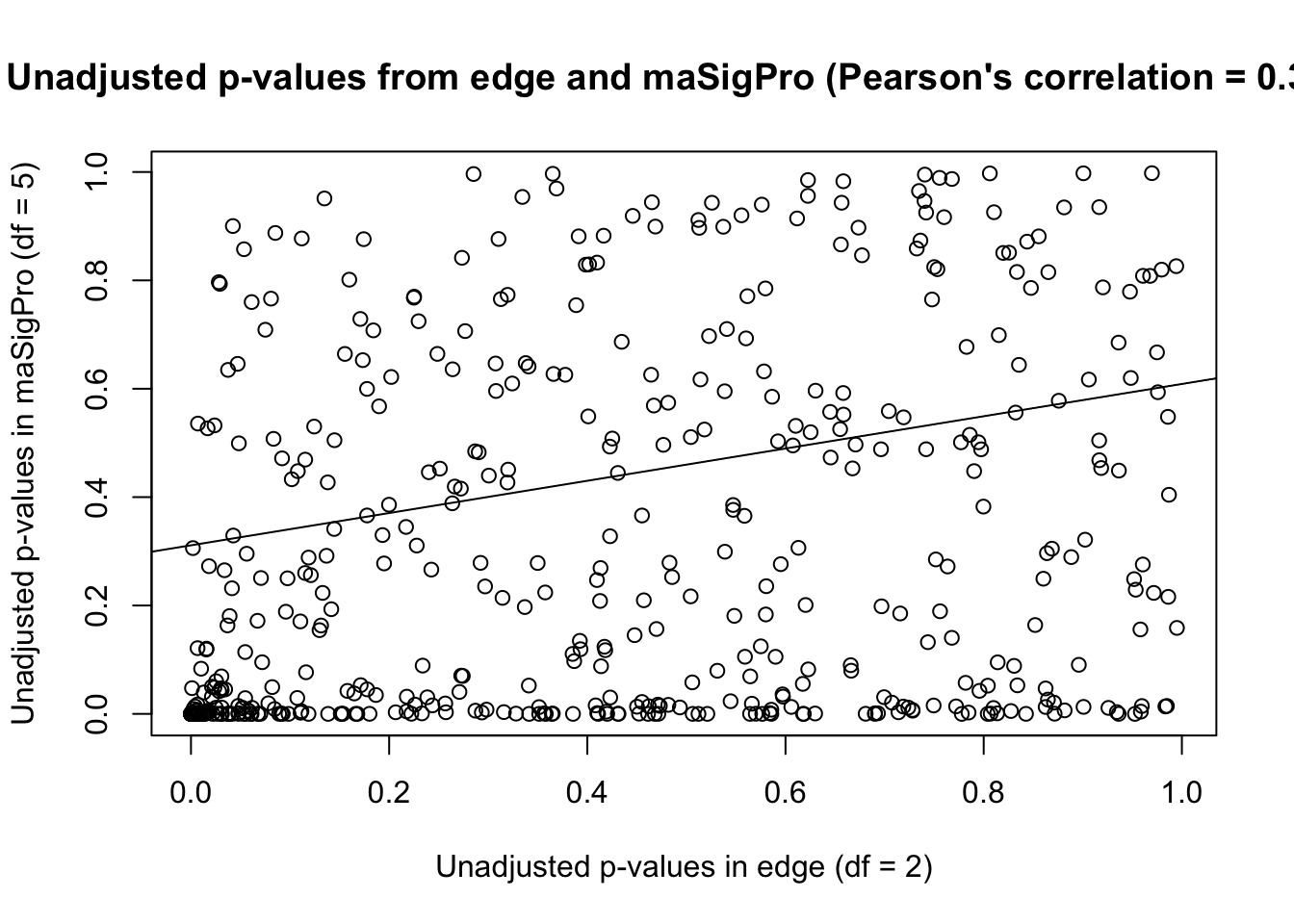
The correlation for unadjusted p-values is higher in edge and maSigPro when df = 2 in maSigPro
Compare Benjamini-Hotchberg corrected p-values from the two software programs
# Make Benjamini-Hotchberg correction for each set of the unadjusted p-values

edge_fdr <- p.adjust(as.matrix(p_value_endo_genes_edge_data), method = "fdr", n = 500)
summary(edge_fdr)
Min. 1st Qu. Median Mean 3rd Qu. Max.
0.0040 0.3300 0.7599 0.6168 0.8855 0.9950 maSigPro_fdr <- p.adjust(as.matrix(p_value_maSigPro_df_2), method = "fdr", n = 500)
summary(maSigPro_fdr) Min. 1st Qu. Median Mean 3rd Qu. Max.
0.00000 0.00473 0.21460 0.34890 0.67860 0.99660 # Combine the two lists of adjusted p-values into one data frame
adjusted_p_value <- as.data.frame(cbind(edge_fdr, maSigPro_fdr))
colnames(adjusted_p_value) <- c("BH adjusted p-values in edge (df = 2)", "BH adjusted p-values in maSigPro (df = 2)")
# Find the correlation between the two numbers
rc <- rcorr(as.matrix(adjusted_p_value), type="pearson") # Correlation = 0.4421 and p equals approximately 0
flattenCorrMatrix(rc$r, rc$P) row
1 BH adjusted p-values in edge (df = 2)
column cor p
1 BH adjusted p-values in maSigPro (df = 2) 0.4229088 0# Compare unadjusted p-values from edge and maSigPro
plot(adjusted_p_value, main = "BH adjusted p-values from edge and maSigPro (Pearson's corr. = 0.4421)")
# Make a best fit line (which we can then add to the plot)
abline(lm(adjusted_p_value[,1] ~ adjusted_p_value[,2]))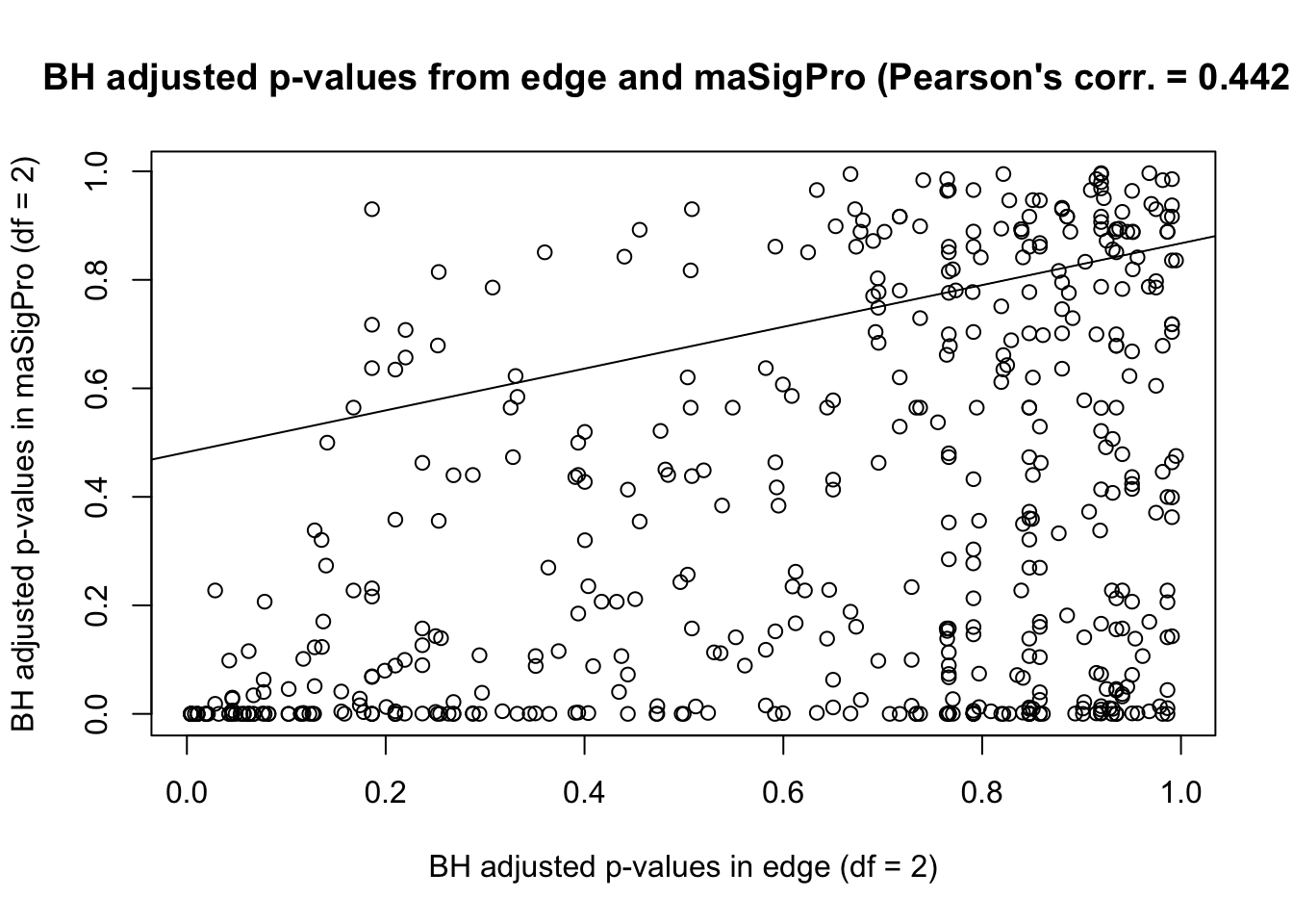
Compare the number of genes at FDR 1% and FDR 10% for both software programs
# Find the number of significant genes at FDR 1%

length(edge_fdr[edge_fdr<=0.01]) # 10 genes
[1] 10length(maSigPro_fdr[maSigPro_fdr<=0.01]) #135 genes[1] 135# Find overlap
overlap_0.01 <- adjusted_p_value[adjusted_p_value[,1] <= 0.01 & adjusted_p_value[,2] <= 0.01, ]
nrow(overlap_0.01)[1] 10# Find the number of significant genes at FDR 10%
length(edge_fdr[edge_fdr<=0.1]) #61 genes[1] 47length(maSigPro_fdr[maSigPro_fdr<=0.1]) # 196 genes[1] 196overlap_0.1 <- adjusted_p_value[adjusted_p_value[,1] <= 0.1 & adjusted_p_value[,2] <= 0.1, ]
nrow(overlap_0.1)[1] 44# Make a table of the results
DF <- data.frame(Program=c("edge", "maSigPro", "Genes in common"), FDR_0.01=c("10", "135", "10"), FDR_0.1=c("61", "196", "55"))
formattable(DF)| Program | FDR_0.01 | FDR_0.1 |
|---|---|---|
| edge | 10 | 61 |
| maSigPro | 135 | 196 |
| Genes in common | 10 | 55 |
Compare the number of DE genes
Compare the p-values and q-values of the genes that were statistically significant in both programs
Session information
R Under development (unstable) (2016-03-11 r70310)
Platform: x86_64-apple-darwin13.4.0 (64-bit)
Running under: OS X 10.10.5 (Yosemite)

locale:
[1] en_US.UTF-8/en_US.UTF-8/en_US.UTF-8/C/en_US.UTF-8/en_US.UTF-8

attached base packages:
[1] stats     graphics  grDevices utils     datasets  methods   base

other attached packages:
[1] formattable_0.2.0.1 Hmisc_3.17-4        ggplot2_2.1.0
[4] Formula_1.2-1       survival_2.39-5     lattice_0.20-33
[7] knitr_1.14

loaded via a namespace (and not attached):
 [1] Rcpp_0.12.6         cluster_2.0.4       magrittr_1.5
 [4] splines_3.3.0       munsell_0.4.3       colorspace_1.2-6
 [7] stringr_1.0.0       plyr_1.8.4          tools_3.3.0
[10] nnet_7.3-12         grid_3.3.0          data.table_1.9.6
[13] gtable_0.2.0        latticeExtra_0.6-28 htmltools_0.3.5
[16] yaml_2.1.13         digest_0.6.10       Matrix_1.2-6
[19] gridExtra_2.2.1     RColorBrewer_1.1-2  formatR_1.4
[22] htmlwidgets_0.7     acepack_1.3-3.3     rpart_4.1-10
[25] evaluate_0.9        rmarkdown_1.0       stringi_1.1.1
[28] scales_0.4.0        chron_2.3-47        foreign_0.8-66